Note
Go to the end to download the full example code.
Run Estimators on a simulated dataset
PyMARE implements a range of meta-analytic estimators. In this example, we build a simulated dataset with a known ground truth and use it to compare PyMARE’s estimators.
Note
The variance of the true effect is composed of both between-study variance
( ) and within-study variance (
 ).
Within-study variance is generally taken from sampling variance values from
individual studies (
).
Within-study variance is generally taken from sampling variance values from
individual studies (v), while between-study variance can be estimated
via a number of methods.
# sphinx_gallery_thumbnail_number = 3
import matplotlib.pyplot as plt
import numpy as np
import seaborn as sns
from scipy import stats

from pymare import core, estimators
from pymare.stats import var_to_ci

sns.set_style("whitegrid")
Here we simulate a dataset
This is a simple dataset with a one-sample design. We are interested in estimating the true effect size from a set of one-sample studies.
N_STUDIES = 40
BETWEEN_STUDY_VAR = 400  # population variance
between_study_sd = np.sqrt(BETWEEN_STUDY_VAR)
TRUE_EFFECT = 20
sample_sizes = np.round(np.random.normal(loc=50, scale=20, size=N_STUDIES)).astype(int)
within_study_vars = np.random.normal(loc=400, scale=100, size=N_STUDIES)
study_means = np.random.normal(loc=TRUE_EFFECT, scale=between_study_sd, size=N_STUDIES)

sample_sizes[sample_sizes <= 1] = 2
within_study_vars = np.abs(within_study_vars)

# Convert data types and match PyMARE nomenclature
y = study_means
X = np.ones((N_STUDIES))
v = within_study_vars
n = sample_sizes
sd = np.sqrt(v * n)
z = y / sd
p = stats.norm.sf(abs(z)) * 2
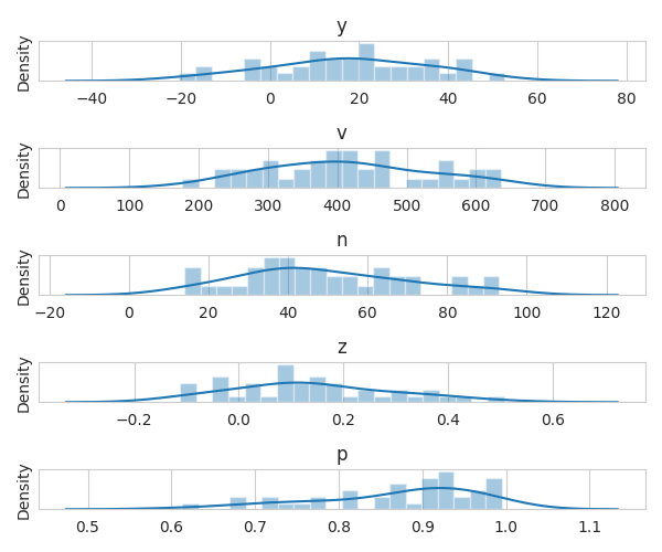
Plot variable distributions
fig, axes = plt.subplots(nrows=5, figsize=(6, 5))
sns.distplot(y, ax=axes[0], bins=20)
axes[0].set_title("y")
sns.distplot(v, ax=axes[1], bins=20)
axes[1].set_title("v")
sns.distplot(n, ax=axes[2], bins=20)
axes[2].set_title("n")
sns.distplot(z, ax=axes[3], bins=20)
axes[3].set_title("z")
sns.distplot(p, ax=axes[4], bins=20)
axes[4].set_title("p")
for i in range(5):
    axes[i].set_yticks([])
fig.tight_layout()
/home/docs/checkouts/readthedocs.org/user_builds/pymare/checkouts/stable/examples/02_meta-analysis/plot_meta-analysis_walkthrough.py:62: UserWarning:

`distplot` is a deprecated function and will be removed in seaborn v0.14.0.

Please adapt your code to use either `displot` (a figure-level function with
similar flexibility) or `histplot` (an axes-level function for histograms).

For a guide to updating your code to use the new functions, please see
https://gist.github.com/mwaskom/de44147ed2974457ad6372750bbe5751

  sns.distplot(y, ax=axes[0], bins=20)
/home/docs/checkouts/readthedocs.org/user_builds/pymare/checkouts/stable/examples/02_meta-analysis/plot_meta-analysis_walkthrough.py:64: UserWarning:

`distplot` is a deprecated function and will be removed in seaborn v0.14.0.

Please adapt your code to use either `displot` (a figure-level function with
similar flexibility) or `histplot` (an axes-level function for histograms).

For a guide to updating your code to use the new functions, please see
https://gist.github.com/mwaskom/de44147ed2974457ad6372750bbe5751

  sns.distplot(v, ax=axes[1], bins=20)
/home/docs/checkouts/readthedocs.org/user_builds/pymare/checkouts/stable/examples/02_meta-analysis/plot_meta-analysis_walkthrough.py:66: UserWarning:

`distplot` is a deprecated function and will be removed in seaborn v0.14.0.

Please adapt your code to use either `displot` (a figure-level function with
similar flexibility) or `histplot` (an axes-level function for histograms).

For a guide to updating your code to use the new functions, please see
https://gist.github.com/mwaskom/de44147ed2974457ad6372750bbe5751

  sns.distplot(n, ax=axes[2], bins=20)
/home/docs/checkouts/readthedocs.org/user_builds/pymare/checkouts/stable/examples/02_meta-analysis/plot_meta-analysis_walkthrough.py:68: UserWarning:

`distplot` is a deprecated function and will be removed in seaborn v0.14.0.

Please adapt your code to use either `displot` (a figure-level function with
similar flexibility) or `histplot` (an axes-level function for histograms).

For a guide to updating your code to use the new functions, please see
https://gist.github.com/mwaskom/de44147ed2974457ad6372750bbe5751

  sns.distplot(z, ax=axes[3], bins=20)
/home/docs/checkouts/readthedocs.org/user_builds/pymare/checkouts/stable/examples/02_meta-analysis/plot_meta-analysis_walkthrough.py:70: UserWarning:

`distplot` is a deprecated function and will be removed in seaborn v0.14.0.

Please adapt your code to use either `displot` (a figure-level function with
similar flexibility) or `histplot` (an axes-level function for histograms).

For a guide to updating your code to use the new functions, please see
https://gist.github.com/mwaskom/de44147ed2974457ad6372750bbe5751

  sns.distplot(p, ax=axes[4], bins=20)
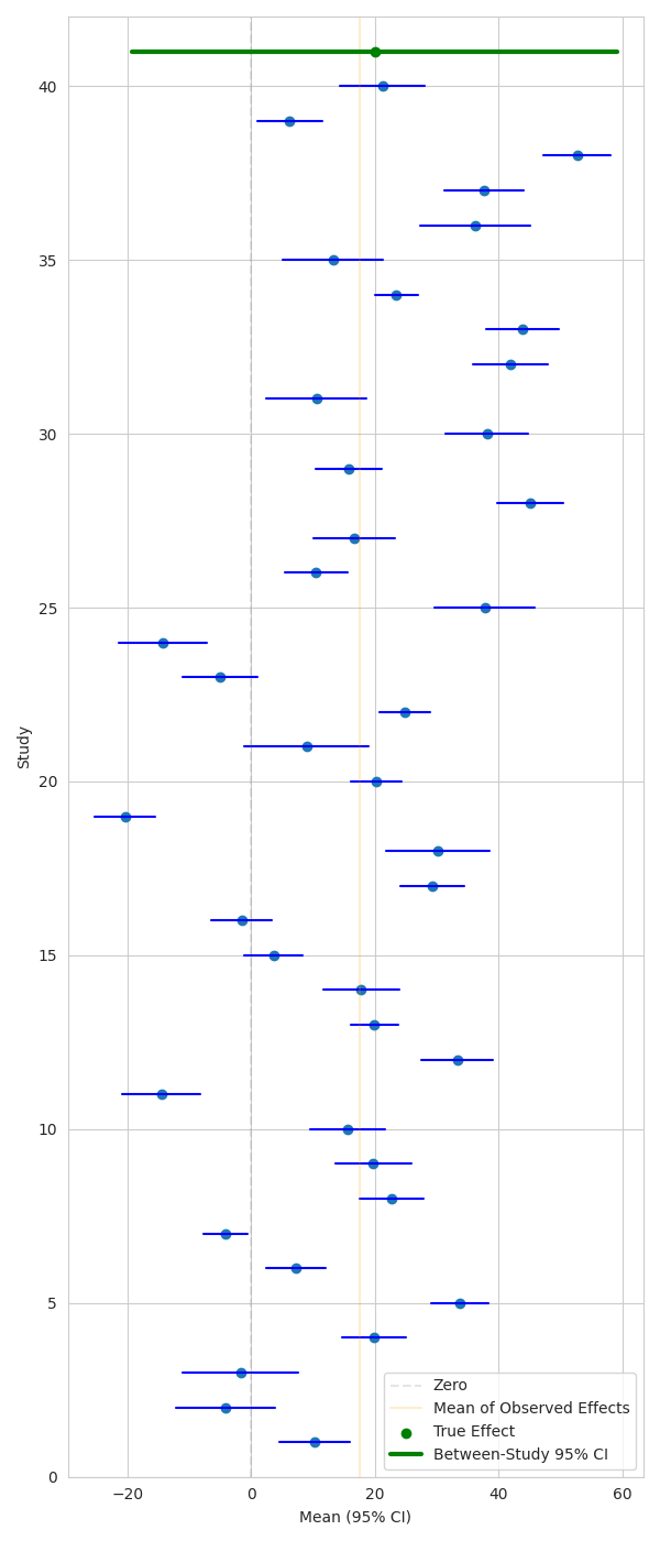
Plot means and confidence intervals
Here we can show study-wise mean effect and CIs, along with the true effect and CI corresponding to the between-study variance.
fig, ax = plt.subplots(figsize=(6, 14))
study_ticks = np.arange(N_STUDIES)

# Get 95% CI for individual studies
lower_bounds, upper_bounds = var_to_ci(y, v, n)
ax.scatter(y, study_ticks + 1)
for study in study_ticks:
    ax.plot((lower_bounds[study], upper_bounds[study]), (study + 1, study + 1), color="blue")
ax.axvline(0, color="gray", alpha=0.2, linestyle="--", label="Zero")
ax.axvline(np.mean(y), color="orange", alpha=0.2, label="Mean of Observed Effects")

# Get 95% CI for true effect
lower_bound, upper_bound = var_to_ci(TRUE_EFFECT, BETWEEN_STUDY_VAR, 1)
ax.scatter((TRUE_EFFECT,), (N_STUDIES + 1,), color="green", label="True Effect")
ax.plot(
    (lower_bound, upper_bound),
    (N_STUDIES + 1, N_STUDIES + 1),
    color="green",
    linewidth=3,
    label="Between-Study 95% CI",
)
ax.set_ylim((0, N_STUDIES + 2))
ax.set_xlabel("Mean (95% CI)")
ax.set_ylabel("Study")
ax.legend()
fig.tight_layout()
Create a Dataset object containing the data
Fit models
When you have z or p:
When you have y and v and don’t want to estimate between-study variance:
When you have y and v and want to estimate between-study variance:
When you have y and n and want to estimate between-study variance:
When you have y and v and want a hierarchical model:
First, we have “combination models”, which combine p and/or z values
The two combination models in PyMARE are Stouffer’s and Fisher’s Tests.
Notice that these models don’t use Dataset objects.
stouff = estimators.StoufferCombinationTest()
stouff.fit(z[:, None])
print("Stouffers")
print("p: {}".format(stouff.params_["p"]))
print()

fisher = estimators.FisherCombinationTest()
fisher.fit(z[:, None])
print("Fishers")
print("p: {}".format(fisher.params_["p"]))
Stouffers
p: [0.18304751]

Fishers
p: [0.87311135]
Now we have a fixed effects model
This estimator does not attempt to estimate between-study variance.
Instead, it takes tau2 () as an argument.
wls = estimators.WeightedLeastSquares()
wls.fit_dataset(dset)
wls_summary = wls.summary()
results["Weighted Least Squares"] = wls_summary.to_df()
print("Weighted Least Squares")
print(wls_summary.to_df().T)
Weighted Least Squares
                  0
name      intercept
estimate  17.059549
se         3.021655
z-score    5.645764
p-value         0.0
ci_0.025  11.137215
ci_0.975  22.981883
Methods that estimate between-study variance
The DerSimonianLaird, Hedges, and VarianceBasedLikelihoodEstimator
estimators all estimate between-study variance from the data, and use y
and v.
DerSimonianLaird and Hedges use relatively simple methods for
estimating between-study variance, while VarianceBasedLikelihoodEstimator
can use either maximum-likelihood (ML) or restricted maximum-likelihood (REML)
to iteratively estimate it.
dsl = estimators.DerSimonianLaird()
dsl.fit_dataset(dset)
dsl_summary = dsl.summary()
results["DerSimonian-Laird"] = dsl_summary.to_df()
print("DerSimonian-Laird")
print(dsl_summary.to_df().T)
print()

hedge = estimators.Hedges()
hedge.fit_dataset(dset)
hedge_summary = hedge.summary()
results["Hedges"] = hedge_summary.to_df()
print("Hedges")
print(hedge_summary.to_df().T)
print()

vb_ml = estimators.VarianceBasedLikelihoodEstimator(method="ML")
vb_ml.fit_dataset(dset)
vb_ml_summary = vb_ml.summary()
results["Variance-Based with ML"] = vb_ml_summary.to_df()
print("Variance-Based with ML")
print(vb_ml_summary.to_df().T)
print()

vb_reml = estimators.VarianceBasedLikelihoodEstimator(method="REML")
vb_reml.fit_dataset(dset)
vb_reml_summary = vb_reml.summary()
results["Variance-Based with REML"] = vb_reml_summary.to_df()
print("Variance-Based with REML")
print(vb_reml_summary.to_df().T)
print()

# The ``SampleSizeBasedLikelihoodEstimator`` estimates between-study variance
# using ``y`` and ``n``, but assumes within-study variance is homogenous
# across studies.
sb_ml = estimators.SampleSizeBasedLikelihoodEstimator(method="ML")
sb_ml.fit_dataset(dset)
sb_ml_summary = sb_ml.summary()
results["Sample Size-Based with ML"] = sb_ml_summary.to_df()
print("Sample Size-Based with ML")
print(sb_ml_summary.to_df().T)
print()

sb_reml = estimators.SampleSizeBasedLikelihoodEstimator(method="REML")
sb_reml.fit_dataset(dset)
sb_reml_summary = sb_reml.summary()
results["Sample Size-Based with REML"] = sb_reml_summary.to_df()
print("Sample Size-Based with REML")
print(sb_reml_summary.to_df().T)
DerSimonian-Laird
                  0
name      intercept
estimate  17.324576
se         3.367076
z-score    5.145289
p-value         0.0
ci_0.025  10.725229
ci_0.975  23.923923

Hedges
                   0
name       intercept
estimate   17.256259
se          0.158114
z-score   109.138162
p-value          0.0
ci_0.025   16.946361
ci_0.975   17.566156

Variance-Based with ML
                  0
name      intercept
estimate  17.324576
se         3.367077
z-score    5.145287
p-value         0.0
ci_0.025  10.725226
ci_0.975  23.923925

Variance-Based with REML
                  0
name      intercept
estimate  17.358699
se         3.419877
z-score    5.075825
p-value         0.0
ci_0.025  10.655863
ci_0.975  24.061534

Sample Size-Based with ML
                  0
name      intercept
estimate  18.512888
se         3.292117
z-score      5.6234
p-value         0.0
ci_0.025  12.060458
ci_0.975  24.965319

Sample Size-Based with REML
                  0
name      intercept
estimate  17.089503
se         3.531874
z-score     4.83865
p-value    0.000001
ci_0.025  10.167157
ci_0.975  24.011849
What about the Stan estimator?
We’re going to skip this one here because of how computationally intensive it is.
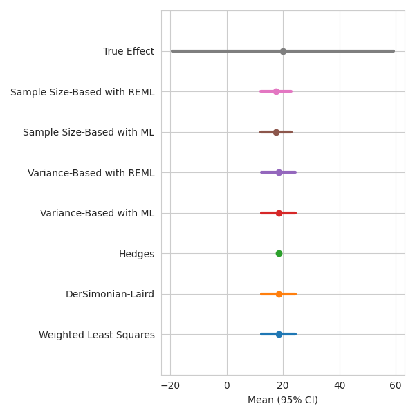
Let’s check out our results!
fig, ax = plt.subplots(figsize=(6, 6))

for i, (estimator_name, summary_df) in enumerate(results.items()):
    ax.scatter((summary_df.loc[0, "estimate"],), (i + 1,), label=estimator_name)
    ax.plot(
        (summary_df.loc[0, "ci_0.025"], summary_df.loc[0, "ci_0.975"]),
        (i + 1, i + 1),
        linewidth=3,
    )

# Get 95% CI for true effect
lower_bound, upper_bound = var_to_ci(TRUE_EFFECT, BETWEEN_STUDY_VAR, 1)
ax.scatter((TRUE_EFFECT,), (i + 2,), label="True Effect")
ax.plot(
    (lower_bound, upper_bound),
    (i + 2, i + 2),
    linewidth=3,
    label="Between-Study 95% CI",
)
ax.set_ylim((0, i + 3))
ax.set_yticklabels([None] + list(results.keys()) + ["True Effect"])

ax.set_xlabel("Mean (95% CI)")
fig.tight_layout()
/home/docs/checkouts/readthedocs.org/user_builds/pymare/checkouts/stable/examples/02_meta-analysis/plot_meta-analysis_walkthrough.py:261: UserWarning: set_ticklabels() should only be used with a fixed number of ticks, i.e. after set_ticks() or using a FixedLocator.
  ax.set_yticklabels([None] + list(results.keys()) + ["True Effect"])
Total running time of the script: (0 minutes 0.746 seconds)